cog | Micro Graph Database for Python. Lives inside your Python process. Quick setup. No server. Runs in notebooks, apps, even your browser.

A persistent graph database that lives inside your Python process.
Quick setup. No server. Runs in notebooks, apps, even your browser.

Quick Start

pip install cogdb

from cog.torque import Graph

# Create a graph and add data
g = Graph("social")
g.put("alice", "follows", "bob")
g.put("bob", "follows", "charlie")
g.put("bob", "status", "active")

# Query
g.v("alice").out("follows").all()                    # → {'result': [{'id': 'bob'}]}
g.v().has("status", "active").all()                  # → {'result': [{'id': 'bob'}]}
g.v("alice").out("follows").out("follows").all()     # → {'result': [{'id': 'charlie'}]}

# Serve your graph over HTTP
g.serve()  # Now queryable at http://localhost:8080

# Expose to the internet with ngrok
# $ ngrok http 8080
# Query your graph from anywhere: https://your-ngrok-url.ngrok.io

Full documentation at cogdb.io

Overview

CogDB is a persistent, embedded graph database implemented in Python. It comes with its own graph traversal language called Torque. Torque is a fluent, chainable API that lives in your Python code. There are no query strings and no context switching, you write graph queries the same way you write normal Python.

CogDB is designed to be easy to use and quick to integrate. There is no server to run and no setup overhead. You simply import it into your Python application. CogDB also works well in interactive environments such as IPython and Jupyter notebooks.

CogDB is a triple store. It models data as Node → Edge → Node (eg: Alice → Follows → Bob).

Key-value pairs let you store facts; triples let you store relationships. With a source, a destination, and a label, you get the full expressive power of a graph with only one step more structure than a key-value store.

Documentation

Creating a graph

Using `put` to insert triples

from cog.torque import Graph
g = Graph("people")
g.put("alice","follows","bob")
g.put("bob","follows","fred")
g.put("bob","status","cool_person")
g.put("charlie","follows","bob")
g.put("charlie","follows","dani")
g.put("dani","follows","bob")
g.put("dani","follows","greg")
g.put("dani","status","cool_person")
g.put("emily","follows","fred")
g.put("fred","follows","greg")
g.put("greg","status","cool_person")
g.put("bob","score","5")
g.put("greg","score","10")
g.put("alice","score","7")
g.put("dani","score","100")

Drop Edge

g.drop("bob", "follows", "fred")

Using `putj` to insert JSONs

f = Graph("followers")
f.putj('{"name" : "bob", "status" : "cool_person", "follows" : ["fred", "dani"]}')
f.putj('{"_id":  "1", "name" : "fred", "status" : "cool_person", "follows" : ["alice", "greg"]}')

Using `updatej` to update JSONs

g.updatej('{"_id" : "1", "status" : "not_cool"}')

Torque query examples

Scan vertices

g.scan(3)

{‘result’: [{‘id’: ‘bob’}, {‘id’: ‘emily’}, {‘id’: ‘charlie’}]}

Scan edges

g.scan(3, 'e')

{‘result’: [{‘id’: ‘status’}, {‘id’: ‘follows’}]}

Starting from a vertex, follow all outgoing edges and list all vertices

g.v("bob").out().all()

{‘result’: [{‘id’: ‘5’}, {‘id’: ‘fred’}, {‘id’: ‘cool_person’}]}

Everyone with status ‘cool_person’

g.v().has("status", 'cool_person').all()

{‘result’: [{‘id’: ‘bob’}, {‘id’: ‘dani’}, {‘id’: ‘greg’}]}

Include edges in the results

g.v().has("follows", "fred").inc().all('e')

{‘result’: [{‘id’: ‘dani’, ‘edges’: [‘follows’]}, {‘id’: ‘charlie’, ‘edges’: [‘follows’]}, {‘id’: ‘alice’, ‘edges’: [‘follows’]}]}

starting from a vertex, follow all outgoing edges and count vertices

g.v("bob").out().count()

‘3’

See who is following who and create a view of that network

Note: `render()` is supported only in IPython environment like Jupyter notebook otherwise use view(..).url.

By tagging the vertices ‘from’ and ‘to’, the resulting graph can be visualized.

g.v().tag("from").out("follows").tag("to").view("follows").render()

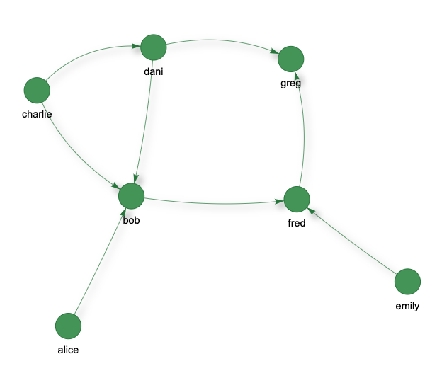
g.v().tag("from").out("follows").tag("to").view("follows").url

file:///Path/to/your/cog_home/views/follows.html

List all views

g.lsv()

[‘follows’]

Load existing visualization

g.getv('follows').render()

starting from a vertex, follow all out going edges and tag them

g.v("bob").out().tag("from").out().tag("to").all()

{‘result’: [{‘from’: ‘fred’, ‘id’: ‘greg’, ‘to’: ‘greg’}]}

starting from a vertex, follow all incoming edges and list all vertices

g.v("bob").inc().all()

{‘result’: [{‘id’: ‘alice’}, {‘id’: ‘charlie’}, {‘id’: ‘dani’}]}

Filtering

g.v().filter(func=lambda x: x.startswith("d")).all()

{‘result’: [{‘id’: ‘dani’}]}

g.v().out("score").filter(func=lambda x: int(x) > 5).inc().all()

{‘result’: [{‘id’: ‘alice’}, {‘id’: ‘dani’}, {‘id’: ‘greg’}]}

g.v("emily").out("follows").filter(func=lambda x: x.startswith("f")).all()

{‘result’: [{‘id’: ‘fred’}]}

Bidirectional Traversal

Follow edges in both directions (outgoing and incoming):

g.v("bob").both("follows").all()

{‘result’: [{‘id’: ‘fred’}, {‘id’: ‘alice’}, {‘id’: ‘charlie’}, {‘id’: ‘dani’}]}

Filter to Specific Nodes

Filter results to only include specific vertices:

g.v("alice").out("follows").is_("bob", "dani").all()

{‘result’: [{‘id’: ‘bob’}, {‘id’: ‘dani’}]}

Remove Duplicates

Remove duplicate vertices from results:

g.v().out("follows").unique().all()

{‘result’: [{‘id’: ‘bob’}, {‘id’: ‘fred’}, {‘id’: ‘greg’}, {‘id’: ‘dani’}]}

Pagination with Limit and Skip

Limit results to first N vertices:

g.v().limit(3).all()

{‘result’: [{‘id’: ‘alice’}, {‘id’: ‘bob’}, {‘id’: ‘charlie’}]}

Skip first N vertices:

g.v().skip(2).limit(2).all()

{‘result’: [{‘id’: ‘charlie’}, {‘id’: ‘dani’}]}

Navigate Back to Tagged Vertex

Return to a previously tagged position while preserving the traversal path:

g.v("alice").tag("start").out("follows").out("follows").back("start").all()

{‘result’: [{‘start’: ‘alice’, ‘id’: ‘alice’}]}

BFS and DFS Traversal

Breadth-first search (level by level, finds shortest paths):

g.v("alice").bfs(predicates="follows", max_depth=2).all()

{‘result’: [{‘id’: ‘bob’}, {‘id’: ‘charlie’}]}

Depth-first search (explores deep before backtracking):

g.v("alice").dfs(predicates="follows", max_depth=3).all()

Filter by depth range:

# Only vertices at exactly depth 2
g.v("alice").bfs(max_depth=2, min_depth=2).all()

Stop at a target:

g.v("alice").bfs(until=lambda v: v == "fred").all()

Bidirectional traversal:

g.v("bob").bfs(direction="both", max_depth=2).all()

Using `put_batch` for bulk inserts (faster)

from cog.torque import Graph
g = Graph("people")

# Insert multiple triples at once - significantly faster for large graphs
g.put_batch([
    ("alice", "follows", "bob"),
    ("bob", "follows", "charlie"),
    ("charlie", "follows", "alice"),
    ("alice", "likes", "pizza"),
    ("bob", "likes", "tacos"),
])

Performance Tuning

Control flush behavior for faster bulk inserts:

# Default: flush every write (safest)
g = Graph("mydb")

# Fast mode: flush every 100 writes (auto-enables async)
g = Graph("mydb", flush_interval=100)

# Manual flush only (fastest for bulk loads)
g = Graph("mydb", flush_interval=0)
g.put_batch(large_dataset)
g.sync()  # Flush when done

`flush_interval`	Behavior	Use Case
`1` (default)	Flush every write	Interactive, safe
`> 1`	Async flush every N writes	Bulk inserts
`0`	Manual only (`sync()`)	Maximum speed

Serving a Graph Over Network

Serve a graph over HTTP and query it from another process or machine:

from cog.torque import Graph

# Create and serve a graph
g = Graph("social")
g.put("alice", "follows", "bob")
g.put("bob", "follows", "charlie")
g.serve(port=8080)

Query from another Python process:

from cog.torque import Graph

# Connect to remote graph
remote = Graph.connect("http://localhost:8080/social")

# Query just like a local graph
remote.v("alice").out("follows").all()
# {'result': [{'id': 'bob'}]}

Stop the server:

g.stop()

json example

#### Using `putj` to insert JSONs
f = Graph("followers")
f.putj('{"name" : "bob", "status" : "cool_person", "follows" : ["fred", "dani"]}')
f.putj('{"name" : "fred", "status" : "cool_person", "follows" : ["alice", "greg"]}')

f.v().has('name','bob').out('follows').all()

{‘result’: [{‘id’: ‘dani’}, {‘id’: ‘fred’}]}

f.v().has('name','fred').out('follows').all()

{‘result’: [{‘id’: ‘greg’}, {‘id’: ‘alice’}]}

In a json, CogDB treats _id property as a unique identifier for each object. If _id is not provided, a randomly generated _id is created for each object with in a JSON object. _id field is used to update a JSON object, see example below.

Using word embeddings

CogDB supports word embeddings with SIMD-optimized similarity search powered by SimSIMD. Word embeddings are useful for semantic search, recommendations, and NLP tasks.

Load pre-trained embeddings (GloVe):

# Load GloVe embeddings (one-liner!)
count = g.load_glove("glove.6B.100d.txt", limit=50000)
print(f"Loaded {count} embeddings")

Load from Gensim model:

from gensim.models import Word2Vec
model = Word2Vec(sentences)
count = g.load_gensim(model)

Add embeddings manually:

from cog.torque import Graph
g = Graph("fruits")

# Add items to graph AND store their embeddings
g.put("orange", "type", "citrus")
g.put("tangerine", "type", "citrus")
g.put("apple", "type", "pome")
g.put("banana", "type", "tropical")

g.put_embedding("orange", [0.9, 0.8, 0.2, 0.1])
g.put_embedding("tangerine", [0.85, 0.75, 0.25, 0.15])
g.put_embedding("apple", [0.5, 0.5, 0.5, 0.5])
g.put_embedding("banana", [0.2, 0.3, 0.8, 0.7])

Find k-nearest neighbors:

# Search within graph vertices
g.v().k_nearest("orange", k=2).all()

{‘result’: [{‘id’: ‘orange’}, {‘id’: ‘tangerine’}]}

# Or search ALL embeddings directly (no g.v() needed)
g.k_nearest("orange", k=2).all()

Filter by similarity threshold:

g.v().sim('orange', '>', 0.9).all()

{‘result’: [{‘id’: ‘tangerine’}, {‘id’: ‘orange’}]}

# Find items in a similarity range
g.v().sim('orange', 'in', [0.5, 0.8]).all()

{‘result’: [{‘id’: ‘apple’}]}

Combine graph traversal with similarity:

# Find citrus fruits similar to orange
g.v().has("type", "citrus").sim("orange", ">", 0.8).all()

{‘result’: [{‘id’: ‘tangerine’}, {‘id’: ‘orange’}]}

Get embedding stats:

g.embedding_stats()

{‘count’: 4, ‘dimensions’: 4}

The sim method filters vertices based on cosine similarity. The k_nearest method returns the top-k most similar vertices.

Loading data from a file

Create a graph from CSV file

from cog.torque import Graph
g = Graph("books")
g.load_csv('test/test-data/books.csv', "book_id")

Get the names of the books that have an average rating greater than 4.0

g.v().out("average_rating", func=lambda x: float(x) > 4.0).inc().out("title").all()

Triples file

CogDB can load a graph stored as N-Triples, a serialization format for RDF. See Wikipedia, W3C for details.

In short, an N-Triple is sequence of subject, predicate and object in a single line that defines a connection between two vertices:

vertex <predicate> vertex

Learn more about RDF triples

from cog.torque import Graph
g = Graph(graph_name="people")
g.load_triples("/path/to/triples.nt", "people")

Edgelist file

from cog.torque import Graph
g = Graph(graph_name="people")
g.load_edgelist("/path/to/edgelist", "people")

Config

If no config is provided when creating a Cog instance, it will use the defaults:

COG_PATH_PREFIX = "/tmp"
COG_HOME = "cog-test"

Example updating config

from cog import config

config.COG_HOME = "app1_home"
data = ('user_data:id=1', '{"firstname":"Hari","lastname":"seldon"}')
cog = Cog(config)
cog.create_or_load_namespace("test")
cog.create_table("db_test", "test")
cog.put(data)
scanner = cog.scanner()
for r in scanner:
 print
 r

Benchmark

Put Perf

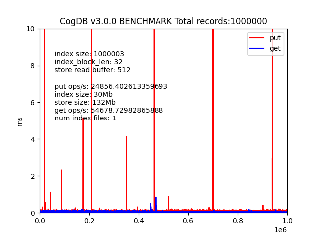
Performance Results

Run benchmarks with: python3 test/benchmark.py

Graph Type	Edges	Speed (edges/s)
Chain (batch)	5,000	4,377
Social network	12,492	3,233
Dense graph	985	2,585
Chain (individual)	5,000	2,712

Batch vs Individual Insert:

1.6x faster at 5,000 edges
Read performance: 20,000+ ops/second